Quantum chemistry and COSMO-SAC screening

Molecules

Thirteen molecules computed from first principles, each one rotatable and traceable to its archived run

Each molecule exactly as the calculation built it: one force-field conformer, then a density-functional surfaceOur calculation

Botanical molecules

Solvents

Caffeine

Formula: C₈H₁₀N₄O₂
Molar mass: 194.19 g/mol
PubChem CID: 2519
Atoms: 24
Surface area: 217 Å²
Donor surface: 2.5%
Acceptor surface: 13.8%
DFT wall time: 246 s

Drag the molecule or use the arrow keys to rotate it. One gas-phase conformer per molecule, not a crystal structure. Shaded zones of the σ-profile: surface able to donate (left) or accept (right) a hydrogen bond.Geometry: RDKit ETKDGv3, 30 conformers (seed 42), MMFF94, lowest energy kept; the DFT surface was computed on this geometry (settings under Provenance). Identity: formulas, molar masses and CIDs from PubChem, retrieved October 24, 2026.

Data table: the 13 computed molecules

The 13 computed molecules: identity (PubChem) and the archived calculation
Molecule	Role	Formula	PubChem CID	Molar mass (g/mol)	Atoms	Surface area (Å²)	Donor surface (%)	Acceptor surface (%)	DFT wall time (s)
Water	Solvent	H₂O	962	18.015	3	43.1	32.5	29.9	1.8
Ethanol	Solvent	C₂H₆O	702	46.07	9	88.9	6.7	11.0	15.2
Acetone	Solvent	C₃H₆O	180	58.08	10	104.0	0.0	13.9	21.4
Ethyl acetate	Solvent	C₄H₈O₂	8857	88.11	14	137.2	0.0	10.1	42.9
n-Hexane	Solvent	C₆H₁₄	8058	86.18	20	160.9	0.0	0.0	62.0
Dichloromethane	Solvent	CH₂Cl₂	6344	84.93	5	100.1	6.4	0.0	6.5
Chloroform	Solvent	CHCl₃	6212	119.37	5	119.4	5.6	0.0	11.9
Carbon tetrachloride	Solvent	CCl₄	5943	153.8	5	138.1	0.0	0.0	11.7
Salicylic acid	Botanical molecule	C₇H₆O₃	338	138.12	16	160.9	5.1	6.0	95.0
Caffeine	Botanical molecule	C₈H₁₀N₄O₂	2519	194.19	24	217.1	2.5	13.8	246.3
Vanillin	Botanical molecule	C₈H₈O₃	1183	152.15	19	186.0	2.2	9.0	117.6
Menthol	Botanical molecule	C₁₀H₂₀O	16666	156.26	31	220.0	2.1	3.7	264.3
Limonene	Botanical molecule	C₁₀H₁₆	440917	136.23	26	205.0	0.0	0.0	193.7

Status. A computational record made with open-source software. EUTECNIQ has no laboratory; measured values come from the cited literature.

Computed surface charge≠a measured property
Low activity coefficient≠high solubility
Screening prediction≠an EUTECNIQ result

COSMO-RS and COSMO-SAC Published methods

This site computes COSMO-SAC, an open variant of COSMO-RS built on the same surface charges

Two models from one surface-charge calculation: COSMO-RS, sold as COSMOtherm, and COSMO-SAC, open code computed herePublished methods

Klamt 1995, J Phys Chem 99:2224–2235; Klamt et al. 1998, J Phys Chem A 102:5074–5085; Eckert & Klamt 2002, AIChE J 48:369–385; BIOVIA COSMOtherm datasheet (Dassault Systèmes, 2024); Lin & Sandler 2002, Ind Eng Chem Res 41:899–913; Hsieh, Sandler & Lin 2010, Fluid Phase Equilib 297:90–97; Bell et al. 2020, J Chem Theory Comput 16:2635–2646, and github.com/usnistgov/COSMOSAC (MIT license). Read October 24, 2026.

Explanation, details and sources

No COSMO-RS calculation was run for this site and no licensed software is used; every COSMO-SAC number here can be regenerated from the archived scripts.

COSMO-RS (conductor-like screening model for real solvents) was introduced by Klamt in 1995 and refined and parameterized in 1998. It combines a quantum-chemistry calculation of each molecule in a perfect conductor with statistical thermodynamics of interacting surface segments, and needs no experimental mixture data (Eckert & Klamt 2002). Its commercial implementation is BIOVIA COSMOtherm (Dassault Systèmes), which reads one COSMO file per compound.

COSMO-SAC (segment activity coefficient) was proposed by Lin and Sandler in 2002 as an activity-coefficient model based on COSMO-RS: the same screening charges, with each molecule treated as a collection of surface segments whose activity coefficients sum to the molecule's. It needs one radius per atom and three universal parameters. The 2010 revision (Hsieh, Sandler & Lin) uses separate σ-profiles for different hydrogen-bonding groups and a temperature-dependent electrostatic term.

Why COSMO-SAC here: its equations, universal constants and a benchmark open-source implementation (NIST; Bell et al. 2020, MIT license) are published, so every number can be checked line by line and regenerated. Our surfaces use the COSMO-RS atomic radii (Klamt et al. 1998) and open-source PySCF; the COSMO-SAC constants were fitted to surfaces from a different quantum-chemistry setup, so the results are a screening-level ranking.

Method in brief

Seven steps lead from a structure to a predicted solubility, and the last one needs measured data

Salicylic acid through all seven steps, from SMILES to predicted solubilityOur calculation

Panels 2–4 project the archived 3D geometry and surface onto the ring plane (top face shown). Measured solubility: Shalmashi & Eliassi 2008; fusion data: NIST Chemistry WebBook.COSMO: Klamt & Schüürmann 1993. COSMO-RS: Klamt 1995. COSMO-SAC: Lin & Sandler 2002; Hsieh, Sandler & Lin 2010; open benchmark implementation: Bell et al. 2020.

Text version of the seven steps

Steps 2 to 4 are quantum chemistry; steps 5 and 6 are statistical thermodynamics, the bookkeeping of which surfaces touch in a liquid.

StructureA SMILES string becomes 3D conformers; the lowest-energy force-field shape is kept.
Electron densityDensity functional theory (BP86/def2-SVP) computes the molecule's electron cloud.
Perfect conductorThe molecule sits in a cavity inside an ideal conductor (ε → ∞).
Surface chargesThe conductor answers with a screening charge density σ on every surface patch.
σ-profileSurface area at each σ level: the molecule's polarity fingerprint.
Activity coefficientCOSMO-SAC pairs solute and solvent patches and returns γ, how welcome a molecule is.
Solubilityγ plus the crystal's melting point and heat of fusion gives a mole-fraction solubility.

Beyond the model's universal constants, the only measured inputs are two numbers per solid: melting temperature and heat of fusion.

Steps 1 to 4, live

Polar hydrogens show blue, oxygen and nitrogen show red, and hydrocarbon surface stays near neutral

Computed screening-charge surfaces (BP86/def2-SVP in a perfect conductor)Our calculation

Drag to rotate

−0.020+0.02 e/Å²

Blue, σ below zero. Faces a positive part of the molecule, usually an O–H or N–H hydrogen. Can donate a hydrogen bond.
Light, σ near zero. Carbon–hydrogen and carbon surface. Nonpolar.
Red, σ above zero. Faces an electron-rich atom such as oxygen or nitrogen. Can accept a hydrogen bond.

43 Å²surface area

25 Å³volume inside the surface

33%of the area is blue enough to donate a hydrogen bond

30%of the area is red enough to accept one

Water. About 62% of its tiny surface is charged enough to donate or accept a hydrogen bond, by far the highest share on this page.

Drag to rotate. Every dot is one surface patch, colored by its screening charge density σ.Surfaces computed for this page with PySCF 2.14.0 (Sun et al. 2018, 2020): BP86 functional (Becke 1988; Perdew 1986), def2-SVP basis (Weigend & Ahlrichs 2005), C-PCM with infinite dielectric constant (the COSMO conductor limit), COSMO-RS atomic radii (Klamt et al. 1998), smooth surface discretization (York & Karplus 1999). Geometries: RDKit conformer search (Riniker & Landrum 2015) with MMFF94 (Halgren 1996); a single DFT calculation on the force-field geometry, without quantum-mechanical geometry optimization. Points are thinned for display; σ is shown after the standard local averaging (Mullins et al. 2006).

What each computed surface shows (all 13 molecules)

Molecule	What the computed surface shows
Water	About 62% of its tiny surface is charged enough to donate or accept a hydrogen bond, by far the highest share on this page.
Ethanol	One O–H group on a small hydrocarbon body: about 18% of the surface can form hydrogen bonds, the rest is nonpolar.
Acetone	Its C=O oxygen gives an acceptor patch (14% of the surface). Nothing on it can donate a hydrogen bond.
Ethyl acetate	The ester oxygens give acceptor patches (10% of the surface). No donor surface.
n-Hexane	Nonpolar everywhere: no patch comes near either hydrogen-bond threshold.
Dichloromethane	Two C–H hydrogens, polarized by the chlorines, form a small donor patch (6% of the surface). The chlorines stay close to neutral.
Chloroform	Its single C–H hydrogen, pulled by three chlorines, forms a small donor patch (6% of the surface).
Carbon tetrachloride	Symmetric and nonpolar: every patch stays close to neutral.
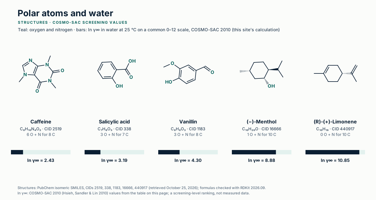
Salicylic acid	The phenol O–H is bonded to the acid's own C=O inside the molecule, so almost all of the donor surface comes from the acid O–H. About 11% of the area passes a threshold.
Caffeine	Two C=O oxygens and one ring nitrogen give acceptor patches (14% of the surface). It has no O–H or N–H; its small donor patch (3%) is a ring C–H.
Vanillin	The aldehyde oxygen carries most of the acceptor surface. The phenol O–H points at the neighboring methoxy oxygen, leaving a small donor patch (2%).
Menthol	One O–H on a large hydrocarbon ring: only about 6% of the surface can form hydrogen bonds.
Limonene	A hydrocarbon terpene: no patch comes near either hydrogen-bond threshold.

Donor and acceptor shares, areas and volumes for every molecule are in the descriptor table under Provenance.

About 62% of water's surface can form hydrogen bonds and none of hexane's can, which is why the model predicts they barely mix.

Step 5

The σ-profile shows how much of the surface sits at each charge level

σ-profiles from our calculations (share of each molecule's surface per 0.001 e/Å² step)Our calculation

Pick up to four molecules. Peaks in the shaded zones mean hydrogen-bonding surface.Shaded zones: |σ| above 0.0084 e/Å², the hydrogen-bond threshold used in COSMO-SAC (Lin & Sandler 2002; Mullins et al. 2006). Binning: 51 bins from −0.025 to +0.025 e/Å² with the area split between the two nearest bins (Mullins et al. 2006). Our water profile shows the expected two peaks, near −0.013 and +0.015 e/Å².

Show data: σ-profiles of all 13 molecules (surface area per bin, Å²)

σ (e/Å²)	Water	Ethanol	Acetone	Ethyl acet.	Hexane	DCM	Chloroform	CCl₄	Salicylic acid	Caffeine	Vanillin	Menthol	Limonene
−0.025	0.00	0.00	0.00	0.00	0.00	0.00	0.00	0.00	0.00	0.00	0.00	0.00	0.00
−0.024	0.00	0.00	0.00	0.00	0.00	0.00	0.00	0.00	0.00	0.00	0.00	0.00	0.00
−0.023	0.00	0.00	0.00	0.00	0.00	0.00	0.00	0.00	0.00	0.00	0.00	0.00	0.00
−0.022	0.00	0.00	0.00	0.00	0.00	0.00	0.00	0.00	0.00	0.00	0.00	0.00	0.00
−0.021	0.00	0.00	0.00	0.00	0.00	0.00	0.00	0.00	0.00	0.00	0.00	0.00	0.00
−0.020	0.00	0.00	0.00	0.00	0.00	0.00	0.00	0.00	0.00	0.00	0.00	0.00	0.00
−0.019	0.00	0.00	0.00	0.00	0.00	0.00	0.00	0.00	0.17	0.00	0.00	0.00	0.00
−0.018	0.00	0.00	0.00	0.00	0.00	0.00	0.00	0.00	0.96	0.00	0.00	0.00	0.00
−0.017	0.00	0.00	0.00	0.00	0.00	0.00	0.00	0.00	1.09	0.00	0.00	0.00	0.00
−0.016	0.00	0.02	0.00	0.00	0.00	0.00	0.00	0.00	0.61	0.00	0.00	0.00	0.00
−0.015	0.35	0.81	0.00	0.00	0.00	0.00	0.00	0.00	1.09	0.00	0.15	0.00	0.00
−0.014	2.73	1.14	0.00	0.00	0.00	0.00	0.00	0.00	0.54	0.00	0.65	0.38	0.00
−0.013	2.87	1.08	0.00	0.00	0.00	0.00	0.39	0.00	0.60	0.00	0.55	0.80	0.00
−0.012	2.89	0.71	0.00	0.00	0.00	0.00	2.18	0.00	0.88	0.00	0.71	0.80	0.00
−0.011	1.68	1.03	0.00	0.00	0.00	0.00	1.65	0.00	0.75	0.00	0.66	0.79	0.00
−0.010	1.58	0.78	0.00	0.00	0.00	1.65	1.34	0.00	0.61	2.33	0.53	0.95	0.00
−0.009	1.66	0.36	0.00	0.00	0.00	4.36	1.24	0.00	0.69	2.87	0.75	0.96	0.00
−0.008	1.19	1.60	0.00	0.00	0.00	3.56	1.26	0.00	1.19	2.64	0.66	1.15	0.00
−0.007	0.99	0.65	2.61	0.71	0.00	4.36	1.16	0.00	3.32	3.97	4.89	1.23	0.00
−0.006	1.02	0.63	10.28	4.20	0.00	3.59	1.43	0.00	7.68	9.02	17.78	1.31	0.00
−0.005	1.36	0.97	8.57	10.63	0.00	3.53	1.23	2.61	9.07	19.26	17.01	1.08	0.00
−0.004	0.96	3.45	10.12	16.12	0.00	1.75	1.52	6.69	9.87	24.48	16.77	2.15	5.79
−0.003	0.73	12.00	11.60	20.83	2.19	3.31	6.68	8.27	11.08	33.49	10.68	9.15	29.95
−0.002	0.46	12.99	12.32	19.14	24.74	4.37	7.88	12.08	11.50	23.21	10.29	40.64	35.90
−0.001	0.57	12.57	13.65	15.78	41.74	5.26	9.61	15.18	10.66	15.95	10.81	46.79	33.24
0.000	1.13	10.35	7.58	11.22	42.59	5.61	11.08	21.41	9.33	9.49	9.17	38.98	35.86
0.001	2.04	7.57	2.11	5.09	30.63	10.98	15.53	48.64	12.68	8.84	13.79	35.59	23.51
0.002	0.71	2.36	0.98	3.04	17.74	6.53	31.38	23.23	14.09	5.78	14.60	18.83	10.61
0.003	0.66	2.23	2.69	3.72	1.26	15.64	23.89	0.00	13.28	5.34	15.89	3.51	7.70
0.004	0.45	1.04	1.62	3.18	0.00	23.39	0.00	0.00	14.00	5.04	10.94	1.76	6.21
0.005	1.38	0.69	0.68	2.73	0.00	2.24	0.00	0.00	5.45	4.42	3.30	1.79	6.40
0.006	1.12	1.42	1.60	2.35	0.00	0.00	0.00	0.00	5.06	4.03	2.70	1.04	5.00
0.007	0.71	1.80	1.04	2.62	0.00	0.00	0.00	0.00	2.57	3.52	3.53	1.38	4.03
0.008	0.90	0.92	2.00	2.77	0.00	0.00	0.00	0.00	3.05	4.36	3.12	1.25	0.85
0.009	2.13	0.75	1.40	1.81	0.00	0.00	0.00	0.00	3.49	4.39	3.95	1.12	0.00
0.010	0.65	1.69	2.40	2.33	0.00	0.00	0.00	0.00	3.48	4.25	3.47	1.08	0.00
0.011	0.85	1.74	3.07	3.67	0.00	0.00	0.00	0.00	2.08	4.25	3.86	1.07	0.00
0.012	2.19	0.81	4.65	4.50	0.00	0.00	0.00	0.00	0.01	8.75	3.59	1.05	0.00
0.013	1.50	1.83	2.69	0.72	0.00	0.00	0.00	0.00	0.00	6.19	1.20	1.35	0.00
0.014	1.85	2.28	0.31	0.00	0.00	0.00	0.00	0.00	0.00	0.62	0.02	1.46	0.00
0.015	2.86	0.59	0.00	0.00	0.00	0.00	0.00	0.00	0.00	0.57	0.00	0.61	0.00
0.016	0.92	0.00	0.00	0.00	0.00	0.00	0.00	0.00	0.00	0.00	0.00	0.00	0.00
0.017	0.00	0.00	0.00	0.00	0.00	0.00	0.00	0.00	0.00	0.00	0.00	0.00	0.00
0.018	0.00	0.00	0.00	0.00	0.00	0.00	0.00	0.00	0.00	0.00	0.00	0.00	0.00
0.019	0.00	0.00	0.00	0.00	0.00	0.00	0.00	0.00	0.00	0.00	0.00	0.00	0.00
0.020	0.00	0.00	0.00	0.00	0.00	0.00	0.00	0.00	0.00	0.00	0.00	0.00	0.00
0.021	0.00	0.00	0.00	0.00	0.00	0.00	0.00	0.00	0.00	0.00	0.00	0.00	0.00
0.022	0.00	0.00	0.00	0.00	0.00	0.00	0.00	0.00	0.00	0.00	0.00	0.00	0.00
0.023	0.00	0.00	0.00	0.00	0.00	0.00	0.00	0.00	0.00	0.00	0.00	0.00	0.00
0.024	0.00	0.00	0.00	0.00	0.00	0.00	0.00	0.00	0.00	0.00	0.00	0.00	0.00
0.025	0.00	0.00	0.00	0.00	0.00	0.00	0.00	0.00	0.00	0.00	0.00	0.00	0.00

Each column sums to the molecule's surface area. Bin centers in e/Å²; DCM is dichloromethane.

Water's surface sits mostly in the two polar zones, hexane's in one peak at zero; the botanical molecules mix a large nonpolar peak with small polar ones.

Step 6, opened up

The σ-potential shows which part of a molecule's surface a solvent penalizes, and the penalties add up to its activity coefficient

Residual part at infinite dilutionln γ_res = (1/a_eff) Σ_σ p_i(σ) ×
[ln Γ_S(σ) − ln Γ_i(σ)]
ln γ∞ = ln γ_res + ln γ_comb

Botanical molecule Solvent

From donor surface (σ < −0.0084)0.36

From nonpolar surface10.35

From acceptor surface (σ > +0.0084)−5.10

Residual part (sum of the bars)5.61

Combinatorial part (size and shape)−3.18

ln γ∞ (matches the heat map below)2.43

γ∞11.4

σ-potential of the solvent (top) and each surface level's contribution to ln γ∞ (bottom), 25 °COur calculation

non-hydrogen-bonding segmentsO–H segmentsother polar segmentsbars: donor surfacenonpolar surfaceacceptor surface

COSMO-SAC 2002 (Lin & Sandler 2002; constants as in Mullins et al. 2006) and 2010 (Hsieh, Sandler & Lin 2010), as implemented on this page from the NIST benchmark code (Bell et al. 2020); σ-profiles from our archived DFT surfaces. Model output, not a measurement.

Method, assumptions and limits

What it calculates: For one botanical molecule infinitely dilute in one pure solvent at 298.15 K, the term each σ bin adds to the residual part of ln γ∞, the three zone sums, the Staverman–Guggenheim combinatorial part and their total.
Equations: Segment activity coefficients of the pure liquid S: ln Γ_S(σ_m) = −ln Σ_n p_S(σ_n) Γ_S(σ_n) exp(−ΔW(σ_m, σ_n)/RT), with p_S the normalized profile; the same for the pure solute i. Each bar is p_i(σ)[ln Γ_S(σ) − ln Γ_i(σ)]/a_eff, with p_i in Å². In the 2010 version the sum also runs over three segment types (non-hydrogen-bonding, O–H, other polar); the bar shows their total at each σ. Combinatorial part: Staverman–Guggenheim term with q = A/79.53 Å², r = V/66.69 Å³, z = 10, at infinite dilution.
Variables and units: σ in e/Å²; a_eff = 7.5 Å² (2002) or 7.25 Å² (2010); ln Γ and ln γ dimensionless; A and V from the archived surfaces.
Assumptions: One conformer per molecule, the archived σ-profiles and both published constant sets exactly as listed under Provenance. Zones use the COSMO-SAC hydrogen-bond threshold 0.0084 e/Å². In the top panel, 2010 O–H and other-polar curves are drawn only where |σ| > 0.005 e/Å², where hydrogen-bonding segments occur.
Valid range: The 5 botanical molecules and 8 solvents computed here, 25 °C, infinite dilution.
What it does not establish: It explains the model's number; it does not make the number right. Solubility also needs the solid's melting properties, and the measured checks are in the next section.
References: Lin & Sandler 2002; Hsieh, Sandler & Lin 2010; Mullins et al. 2006; Bell et al. 2020; Klamt 2005 (σ-potential concept in COSMO-RS).
Verification: The 80 totals (40 pairs × 2 versions) reproduce the archived ln γ∞ within 5.4 × 10⁻⁶. An independent Python script recomputes the readouts from the archived surfaces for 8 cases (tests/numerics/comp-quantum.json).

Water rejects caffeine (ln γ∞ 2.43); the largest single term comes from its nonpolar surface (10.35).

Show data: contributions for all 40 pairs (2010) and the solvent σ-potentials (2002)

COSMO-SAC 2010, 25 °C, infinite dilution: where the residual part of ln γ∞ comes from
Solute	Solvent	Donor surface (σ < −0.0084)	Nonpolar surface	Acceptor surface (σ > +0.0084)	Residual	Combinatorial	ln γ∞
Salicylic acid	Water	−1.66	7.21	−0.47	5.08	−1.89	3.19
Salicylic acid	Ethanol	−2.37	0.46	0.80	−1.12	−0.20	−1.32
Salicylic acid	Acetone	−1.99	−0.81	0.71	−2.08	−0.09	−2.17
Salicylic acid	Ethyl acetate	−1.53	−0.83	0.93	−1.43	0.02	−1.40
Salicylic acid	n-Hexane	3.08	0.10	1.56	4.74	0.03	4.77
Salicylic acid	Dichloromethane	2.24	−0.57	0.84	2.52	−0.13	2.39
Salicylic acid	Chloroform	2.59	−0.64	0.82	2.77	−0.04	2.73
Salicylic acid	CCl₄	2.94	−0.06	1.49	4.37	−0.01	4.36
Caffeine	Water	0.36	10.35	−5.10	5.61	−3.18	2.43
Caffeine	Ethanol	0.17	0.77	−0.14	0.80	−0.56	0.25
Caffeine	Acetone	0.01	−0.11	0.10	−0.00	−0.34	−0.34
Caffeine	Ethyl acetate	0.04	−0.69	0.89	0.24	−0.08	0.17
Caffeine	n-Hexane	0.49	−0.18	3.29	3.61	−0.00	3.61
Caffeine	Dichloromethane	0.18	−1.54	0.18	−1.18	−0.41	−1.59
Caffeine	Chloroform	0.30	−1.43	−0.12	−1.25	−0.23	−1.48
Caffeine	CCl₄	0.44	−0.52	2.95	2.87	−0.13	2.75
Vanillin	Water	−0.07	9.05	−2.20	6.77	−2.47	4.30
Vanillin	Ethanol	−0.41	0.88	0.25	0.72	−0.37	0.35
Vanillin	Acetone	−0.38	−0.38	0.18	−0.57	−0.21	−0.78
Vanillin	Ethyl acetate	−0.20	−0.60	0.59	−0.21	−0.03	−0.24
Vanillin	n-Hexane	1.36	0.43	1.80	3.59	0.01	3.60
Vanillin	Dichloromethane	1.04	−0.68	0.32	0.68	−0.26	0.42
Vanillin	Chloroform	1.17	−0.61	0.22	0.78	−0.12	0.66
Vanillin	CCl₄	1.31	0.17	1.64	3.12	−0.05	3.06
Menthol	Water	0.08	14.18	−2.13	12.14	−3.26	8.88
Menthol	Ethanol	−0.31	1.76	−0.48	0.96	−0.59	0.38
Menthol	Acetone	−0.30	0.86	0.21	0.77	−0.36	0.40
Menthol	Ethyl acetate	−0.11	0.34	0.43	0.66	−0.09	0.57
Menthol	n-Hexane	1.50	−0.39	1.12	2.23	−0.01	2.22
Menthol	Dichloromethane	1.14	0.18	0.19	1.52	−0.44	1.08
Menthol	Chloroform	1.29	−0.39	0.08	0.98	−0.24	0.73
Menthol	CCl₄	1.44	−0.45	1.01	2.00	−0.14	1.87
Limonene	Water	0.00	13.77	−0.00	13.77	−2.92	10.85
Limonene	Ethanol	0.00	2.09	−0.00	2.09	−0.50	1.60
Limonene	Acetone	0.00	1.01	−0.00	1.01	−0.30	0.71
Limonene	Ethyl acetate	0.00	0.58	−0.00	0.57	−0.07	0.51
Limonene	n-Hexane	0.00	0.13	0.00	0.13	−0.00	0.12
Limonene	Dichloromethane	0.00	0.28	−0.00	0.28	−0.36	−0.08
Limonene	Chloroform	0.00	−0.20	−0.00	−0.20	−0.19	−0.39
Limonene	CCl₄	0.00	0.03	0.00	0.03	−0.10	−0.07

Solvent σ-potential, ln Γ_S(σ), COSMO-SAC 2002, 25 °C (every second bin; all 51 bins in the dataset file)
σ (e/Å²)	Water	Ethanol	Acetone	Ethyl acetate	n-Hexane	Dichloromethane	Chloroform	CCl₄
−0.025	−10.84	−9.38	−7.84	−5.56	8.41	6.87	7.56	8.20
−0.023	−9.22	−8.12	−6.92	−4.94	7.13	5.73	6.35	6.93
−0.021	−7.53	−6.79	−5.93	−4.24	5.95	4.71	5.25	5.77
−0.019	−5.79	−5.40	−4.88	−3.48	4.88	3.79	4.26	4.72
−0.017	−4.03	−3.96	−3.78	−2.64	3.92	2.97	3.38	3.77
−0.015	−2.29	−2.50	−2.64	−1.76	3.06	2.26	2.60	2.93
−0.013	−0.70	−1.09	−1.49	−0.86	2.30	1.66	1.92	2.20
−0.011	0.42	0.07	−0.40	−0.04	1.66	1.15	1.36	1.58
−0.009	0.87	0.64	0.41	0.48	1.12	0.75	0.89	1.06
−0.007	0.81	0.54	0.48	0.45	0.68	0.44	0.53	0.64
−0.005	0.71	0.36	0.36	0.31	0.36	0.23	0.27	0.33
−0.003	0.62	0.21	0.23	0.18	0.13	0.10	0.10	0.12
−0.001	0.55	0.11	0.11	0.08	0.02	0.05	0.02	0.02
+0.001	0.48	0.08	0.04	0.03	0.01	0.06	0.03	0.01
+0.003	0.42	0.13	0.03	0.05	0.10	0.13	0.11	0.11
+0.005	0.39	0.25	0.09	0.16	0.31	0.25	0.25	0.31
+0.007	0.39	0.45	0.24	0.35	0.61	0.41	0.42	0.60
+0.009	0.33	0.72	0.49	0.63	1.03	0.60	0.52	1.00
+0.011	−0.17	0.87	0.83	1.02	1.55	0.75	0.09	1.49
+0.013	−1.04	0.56	1.26	1.50	2.18	0.90	−0.70	2.08
+0.015	−2.16	−0.45	1.80	2.08	2.91	1.05	−1.60	2.76
+0.017	−3.39	−1.83	2.43	2.76	3.75	1.20	−2.50	3.54
+0.019	−4.64	−3.31	3.17	3.54	4.70	1.39	−3.36	4.43
+0.021	−5.87	−4.77	4.01	4.42	5.76	1.62	−4.14	5.40
+0.023	−7.07	−6.19	4.95	5.41	6.92	1.93	−4.85	6.48
+0.025	−8.22	−7.55	5.99	6.50	8.19	2.31	−5.48	7.66

Steps 6 and 7

Water pushes out all five botanical molecules, while three ICH Class 3 solvents keep every one below ln γ∞ = 2

How strongly each solvent rejects each botanical molecule: ln γ∞ at 25 °C (COSMO-SAC 2010)Screening-level prediction

strong color: low ln γ∞, the solvent welcomes the moleculefaint: ln γ∞ of 5 or more, the solvent pushes it out

COSMO-SAC 2010 (Hsieh, Sandler & Lin 2010): separate hydrogen-bond terms for O–H groups and for other polar atoms, and an electrostatic term that changes with temperature; surface averaging, profile splitting and constants as in the NIST benchmark code (Bell et al. 2020). The 2002 version (Lin & Sandler 2002, constants as given by Mullins et al. 2006) is in the table and the two charts below. Both constant sets were fitted to a different quantum-chemistry setup, so treat the numbers as a ranking.

Skeletal formulas of caffeine, salicylic acid, vanillin, (−)-menthol and (R)-limonene with oxygen and nitrogen in teal, ordered by the site's COSMO-SAC 2010 prediction of ln γ∞ in water at 25 °C: 2.43, 3.19, 4.30, 8.88 and 10.85. The fewer polar atoms per carbon, the larger the value. — Structures: PubChem isomeric SMILES, CIDs 2519, 338, 1183, 16666, 440917 (retrieved Oct 25, 2026); RDKit 2026.09 2D depiction. ln γ∞: COSMO-SAC 2010 (Hsieh, Sandler & Lin 2010), values from the table on this page. Generated illustration, EUTECNIQ. Full-size SVG

Show data: ln γ∞ for every pair, both model versions

COSMO-SAC 2010

Solute	Water	Ethanol	Acetone	Ethyl acet.	Hexane	DCM	Chloroform	CCl₄
Salicylic acid	3.19	−1.32	−2.17	−1.40	4.77	2.39	2.73	4.36
Caffeine	2.43	0.25	−0.34	0.17	3.61	−1.59	−1.48	2.75
Vanillin	4.30	0.35	−0.78	−0.24	3.60	0.42	0.66	3.06
Menthol	8.88	0.38	0.40	0.57	2.22	1.08	0.73	1.87
Limonene	10.85	1.60	0.71	0.51	0.12	−0.08	−0.39	−0.07

COSMO-SAC 2002

Solute	Water	Ethanol	Acetone	Ethyl acet.	Hexane	DCM	Chloroform	CCl₄
Salicylic acid	1.56	−2.24	−3.58	−2.52	3.20	0.93	0.92	2.85
Caffeine	1.09	−0.54	−0.35	0.22	3.63	−1.93	−5.10	2.87
Vanillin	3.61	0.27	−0.82	−0.25	3.01	−0.24	−1.22	2.53
Menthol	7.56	0.31	0.14	0.32	1.47	0.14	−1.29	1.15
Limonene	9.18	1.34	0.69	0.48	0.11	−0.09	−0.36	−0.07

Natural logarithm of the infinite-dilution activity coefficient of the solute (row) in the solvent (column) at 298.15 K. γ∞ = e^{ln γ∞}; ln γ∞ = 2 means γ∞ ≈ 7.4.

Water pushes out every molecule here (ln γ∞ above 2 in each case), most strongly the two terpenes (ln γ∞ near 9 for menthol and 11 for limonene). Acetone and ethyl acetate suit salicylic acid and vanillin best; caffeine prefers dichloromethane and chloroform; limonene mixes almost ideally with hexane and the chlorinated solvents (ln γ∞ near zero).

In both versions water pushes out every molecule here, the terpenes menthol and limonene most strongly.

Choosing one solvent for all five molecules: drag along any axis to keep only solvents below a ln γ∞ you acceptOur calculation; ICH class verified

Each line is one solvent; lower on every axis is better. Colors: ICH Q3C residual-solvent class, written for medicines and used here only as a published toxicity grouping. Class 3 solvents are acceptable up to 5,000 ppm (50 mg/day) without justification; Class 1 solvents are to be avoided.ln γ∞: our COSMO-SAC screen (table above). ICH Q3C classes and limits: FDA, Q3C — Tables and List, Guidance for Industry, Revision 3 (June 2017).

Data table: ICH Q3C class and ln γ∞ for each solvent

Solvent screen: ICH Q3C class and limit, and ln γ∞ (COSMO-SAC 2010, 25 °C) of each botanical molecule
Solvent	ICH Q3C	Limit (ppm, Option 1)	Salicylic acid	Caffeine	Vanillin	Menthol	Limonene
Water	Not a Q3C solvent	not applicable	3.19	2.43	4.30	8.88	10.85
Ethanol	Class 3	5000	−1.32	0.25	0.35	0.38	1.60
Acetone	Class 3	5000	−2.17	−0.34	−0.78	0.40	0.71
Ethyl acetate	Class 3	5000	−1.40	0.17	−0.24	0.57	0.51
n-Hexane	Class 2	290	4.77	3.61	3.60	2.22	0.12
Dichloromethane	Class 2	600	2.39	−1.59	0.42	1.08	−0.08
Chloroform	Class 2	60	2.73	−1.48	0.66	0.73	−0.39
CCl₄	Class 1	4	4.36	2.75	3.06	1.87	−0.07

In the 2010 version only ethanol, acetone and ethyl acetate stay below ln γ∞ = 2 for all five molecules, and all three are ICH Class 3.

Salicylic acid at 25 °C: predicted versus measured solubility (mole fraction)Measured Prediction

Measured: Shalmashi & Eliassi 2008, J Chem Eng Data 53:199–200 (mass fractions from the NIST TRC ThermoML archive, converted to mole fractions). Fusion data: ΔH_fus = 24.6 kJ/mol at 431.8 K (NIST Chemistry WebBook). Prediction: ideal solubility divided by the COSMO-SAC activity coefficient, solved at the saturated composition (heat-capacity term neglected).

Caffeine at 25 °C: predicted solubility ranking across eight solventsScreening-level prediction

Fusion data: ΔH_fus = 21.9 kJ/mol at 510.2 K, used as T_m (NIST Chemistry WebBook; reported values span 18.3–24.8 kJ/mol; the WebBook T_fus of 509.3 K, used on the thermodynamics page, would change ideal solubility by 0.9%), solid–solid transition ignored. Check: a gravimetric study of eight solvents found caffeine most soluble in chloroform and dichloromethane (Shalmashi & Golmohammad 2010, Lat Am Appl Res 40:283–285). Only that ranking is used here.

Show data: salicylic acid and caffeine solubility

Salicylic acid, 25 °C (mole fraction x)

Solvent	Measured, mass fraction	Measured, x	COSMO-SAC 2010, x	COSMO-SAC 2002, x	2010 ÷ measured	2002 ÷ measured
Water	0.00220	2.87 × 10⁻⁴	2.02 × 10⁻³	0.0129	7.02	44.98
Ethanol	0.3254	0.139	0.124	0.215	0.90	1.55
Ethyl acetate	0.2008	0.138	0.137	0.247	0.99	1.79
Carbon tetrachloride	0.00299	3.33 × 10⁻³	7.62 × 10⁻⁴	3.23 × 10⁻³	0.23	0.97
Acetone	not measured	—	0.195	0.339	—	—
n-Hexane	not measured	—	4.73 × 10⁻⁴	2.17 × 10⁻³	—	—
Dichloromethane	not measured	—	7.78 × 10⁻³	0.0246	—	—
Chloroform	not measured	—	5.20 × 10⁻³	0.0234	—	—

Caffeine, 25 °C (predicted mole fraction x)

Solvent	COSMO-SAC 2010, x	Rank (2010)	COSMO-SAC 2002, x	Rank (2002)
Dichloromethane	0.0804	1	0.0929	2
Chloroform	0.0688	2	0.165	1
Acetone	0.0345	3	0.0349	4
Ethyl acetate	0.0219	4	0.0208	5
Ethanol	0.0197	5	0.0386	3
Water	2.40 × 10⁻³	6	0.0103	6
Carbon tetrachloride	1.67 × 10⁻³	7	1.49 × 10⁻³	7
n-Hexane	6.97 × 10⁻⁴	8	6.87 × 10⁻⁴	8

Ideal solubility (no solvent effect) at 25 °C: salicylic acid x = 0.0464, caffeine x = 0.0254. A ratio above 1 means the model predicts more dissolves than was measured.

For salicylic acid, the 2010 version lands within about 10% of the measured value in ethanol and ethyl acetate, but it is 7 times too high in water and 4 times too low in carbon tetrachloride. The 2002 version is 45 times too high in water. Both versions rank chloroform and dichloromethane first for caffeine, as the measured study found. Good enough to rank solvents; not a substitute for measuring.

For salicylic acid the 2010 version lands within about 10% of measured solubility in ethanol and ethyl acetate but is 7 times too high in water.

Explanation, details and sources

We coded two published versions of the COSMO-SAC model, the 2002 original and its 2010 revision, and ran both on our own surfaces at 25 °C. The model scores every surface contact, then gives each molecule an activity coefficient γ. Below 1, the solvent welcomes it; far above 1, the solvent pushes it out. Values here are at infinite dilution (γ∞), a single solute molecule in pure solvent.

Molecular engineering explorer

A single surface descriptor captures part of a solvent ranking; the full model is needed for the rest

PolarityM₂/A = Σ p(σ) σ² ÷ Σ p(σ)

Polarity mismatch|M₂/A of solute − M₂/A of solvent|; smallest ranks first

Donor and acceptor momentsM_don = Σ p(σ) max(0, −σ − σ_hb); M_acc = Σ p(σ) max(0, σ − σ_hb)

Hydrogen-bond complementarityM_acc(solute)·M_don(solvent) + M_don(solute)·M_acc(solvent); largest ranks first

Rank agreement of the two rankingsρ = Spearman rank correlation
1 = same order
0 = unrelated

Botanical molecule Descriptor that ranks the solvents COSMO-SAC version for the reference ranking

Rank agreement, Spearman ρ (1 = same order)0.90

COSMO-SAC first choiceAcetone (ln γ∞ = −2.17)

Descriptor's first choiceAcetone

Spread of ln γ∞ across the eight solvents6.94

Solvent order for salicylic acid: by descriptor (left) and by COSMO-SAC ln γ∞ (right)Computed comparison

Same position in both rankings, or within one placeMoves two or more places

σ-moments as used in COSMO-RS (Klamt 2005); here computed with the COSMO-SAC hydrogen-bond cut-off. Rankings: lowest ln γ∞ first. Spearman's rank correlation with average ranks for ties.

Method, assumptions and limits

What it calculates: How closely one descriptor, computed from the σ-profiles of the solute and solvent, reproduces the order in which COSMO-SAC ranks eight solvents for one botanical molecule at 25 °C.
Equations: Descriptors as defined above the explorer. Rank agreement ρ = Spearman's rank correlation between the descriptor ranking (most favorable first: smallest mismatch, or largest complementarity) and the COSMO-SAC ranking (lowest ln γ∞ first), with average ranks for ties.
Variables and units: σ in e/Å²; p(σ) in Å²; M₂/A in e²/Å⁴; M_don and M_acc in e; complementarity in e²; ln γ∞ dimensionless.
Assumptions: One conformer per molecule; profiles and ln γ∞ exactly as in the tables on this page; σ_hb = 0.0084 e/Å². Both rankings are computed from our σ-profiles; neither is a measurement. With eight solvents, swapping two neighbors in one ranking changes ρ by 0.024. Descriptors ignore temperature, molecular size and competition between patches; COSMO-SAC includes them.
Valid range: The five botanical molecules and eight solvents computed here, at 298.15 K. ρ is not defined when a descriptor has the same value for every solvent (limonene has no hydrogen-bonding surface, so its complementarity is zero everywhere).
What it does not establish: It does not test either ranking against measurements, and it does not show that any descriptor predicts solubility. Solubility also depends on the solid's melting properties and on concentration.
References: Klamt A. COSMO-RS: From Quantum Chemistry to Fluid Phase Thermodynamics and Drug Design. Elsevier; 2005. Lin & Sandler 2002; Hsieh, Sandler & Lin 2010; Bell et al. 2020.
Verification: An independent Python script recomputes the descriptors from the archived full-precision profiles and the Spearman coefficients with SciPy; the page values are checked against it for 8 cases (tests/numerics/insights-quantum-chemistry.json).

Polarity mismatch alone nearly reproduces the model's solvent order for vanillin (ρ = 1.00) and salicylic acid (0.90), but not for caffeine (0.50) or menthol (−0.10).

Show data: rank agreement for every molecule, descriptor and model version

Polarity mismatch orders the eight solvents almost as COSMO-SAC 2010 does for vanillin (ρ = 1.00), salicylic acid (0.90) and limonene (0.81), but not for caffeine (0.50) or menthol (−0.10). Hydrogen-bond complementarity agrees less (ρ from 0.06 to 0.59; not defined for limonene, which has no hydrogen-bonding surface). Water offers caffeine the most hydrogen-bond partners (4.6 × 10⁻³ e²), yet the model predicts it rejects caffeine (ln γ∞ = 2.4): in the model, water's donor and acceptor patches pair with each other more favorably than with caffeine's.

Botanical molecule	Polarity mismatch, 2010	H-bond complementarity, 2010	Polarity mismatch, 2002	H-bond complementarity, 2002
Salicylic acid	0.90	0.59	0.88	0.61
Caffeine	0.50	0.37	0.55	0.56
Vanillin	1.00	0.06	0.74	0.08
Menthol	−0.10	0.30	0.48	0.11
Limonene	0.81	not defined	0.81	not defined

Polarity mismatch, 10⁻⁵ e²/Å⁴ (botanical molecule against each solvent)

Botanical molecule	Water	Ethanol	Acetone	Ethyl acet.	Hexane	DCM	Chloroform	CCl₄
Salicylic acid	7.73	0.56	0.26	0.58	2.70	1.01	1.60	2.55
Caffeine	7.30	0.14	0.16	1.00	3.13	1.43	2.03	2.97
Vanillin	7.85	0.68	0.39	0.46	2.58	0.89	1.48	2.42
Menthol	9.39	2.22	1.93	1.08	1.04	0.66	0.06	0.88
Limonene	9.93	2.77	2.47	1.63	0.50	1.20	0.60	0.34

Hydrogen-bond complementarity, 10⁻³ e²

Botanical molecule	Water	Ethanol	Acetone	Ethyl acet.	DCM	Chloroform
Salicylic acid	3.12	1.90	1.94	1.51	0.07	0.22
Caffeine	4.61	2.26	0.24	0.19	0.46	1.48
Vanillin	2.50	1.31	0.55	0.43	0.19	0.61
Menthol	2.06	1.10	0.56	0.44	0.14	0.46
Limonene	0.00	0.00	0.00	0.00	0.00	0.00

Explanation, details and sources

Formulators often reason with one number, such as polarity. Here two such descriptors, computed from the same σ-profiles, are compared with the full COSMO-SAC ranking of eight solvents for each botanical molecule. Both sides of this comparison are computed; the check against measurement is the salicylic acid chart above.

p(σ) is the area in each σ bin of a σ-profile; σ_hb = 0.0084 e/Å², the COSMO-SAC hydrogen-bond threshold.

Provenance

Every number on this page can be regenerated from the archived scripts

Eight archived steps, each re-run on October 22, 2026 with the same result to within numerical noiseOur calculation

Scripts and full surfaces are archived with the site source and available on request; structures, settings, σ-profiles and screening results download as one file: qc-dataset.json (JSON, 40 KB). Screening results compared by relative difference. Every constant was checked line by line against NIST's COSMO-SAC code; the UD and VT-2005 σ-profile databases distributed with it were not used (academic, non-commercial license).Bell et al. 2020 (github.com/usnistgov/COSMOSAC, commit 1b82456); Klamt et al. 1998 (radii); Mullins et al. 2006; NIST Chemistry WebBook.

The 13 computed moleculesPubChem-matched structures

Structures drawn from the SMILES in the table below; each RDKit InChIKey matches the PubChem record (CIDs 962, 702, 180, 8857, 8058, 6344, 6212, 5943, 338, 2519, 1183, 16666, 440917; checked October 23, 2026).

Text version: re-run result and calculation settings

Reproducibility check. On October 22, 2026, all 13 surface calculations and the COSMO-SAC screen were re-run from the archived scripts in a fresh copy of the folder. Geometries were identical, total energies agreed within 4 × 10⁻¹² E_h, σ-profiles within 2 × 10⁻¹⁰ Å² per bin, and all 123 screening results within a relative 4 × 10⁻¹¹.

Calculation settings

Structures: 13 molecules entered as SMILES (table below). Stereocenters as written: (1R,2S,5R)-menthol and (R)-limonene, by RDKit's CIP labeling.
Conformers: RDKit ETKDGv3 distance-geometry embedding, 30 conformers per molecule (random seed 42; one for water), each minimized with MMFF94 (up to 2,000 iterations; all converged). The lowest-energy conformer is used. No quantum-mechanical geometry optimization.
Electronic structure: PySCF 2.14.0, restricted Kohn–Sham DFT, BP86 functional (Becke 1988 exchange, Perdew 1986 correlation), def2-SVP basis with density fitting, integration grid level 2.
Convergence: Gas-phase SCF to PySCF's default energy tolerance of 10⁻⁹ E_h; conductor SCF to 10⁻⁸ E_h, started from the gas-phase density. All 26 SCF runs converged.
Conductor model: C-PCM with the dielectric constant set to infinity (the COSMO conductor limit); smooth (SWIG) surface discretization with a 194-point Lebedev grid per atom; radii H 1.30, C 2.00, N 1.83, O 1.72, Cl 2.05 Å (Klamt et al. 1998).
Surface charge density: σ = screening charge ÷ segment area, in e/Å²; positive σ faces electron-rich atoms. Cavity volume from the surface by the divergence theorem. Net screening charge near zero (−0.005 to −0.035 e) confirms that the cavity captured almost all of each molecule's field.
Averaging and σ-profile: 2002 version: local averaging radius 0.81764 Å, decay factor 1 (Mullins et al. 2006). 2010 version: radius (7.25/π)^½ Å, decay factor 3.57, profile split into non-hydrogen-bonding, O–H and other polar parts with P_hb(σ) = 1 − exp(−σ²/2σ₀²), σ₀ = 0.007 e/Å². 51 bins from −0.025 to +0.025 e/Å², area split linearly between neighboring bins.
COSMO-SAC 2002 constants: α′ = 16,466.72 and c_hb = 85,580 kcal·Å⁴/(mol·e²); σ_hb = 0.0084 e/Å²; a_eff = 7.5 Å²; q₀ = 79.53 Å², r₀ = 66.69 Å³, z = 10.
COSMO-SAC 2010 constants: A_ES = 6,525.69 kcal·Å⁴/(mol·e²), B_ES = 1.4859 × 10⁸ kcal·Å⁴·K²/(mol·e²); c_OH–OH = 4,013.78, c_OT–OT = 932.31, c_OH–OT = 3,016.43 kcal·Å⁴/(mol·e²); a_eff = 7.25 Å². No dispersion term.
Source of the constants: Re-implemented in Python from NIST's open-source COSMO-SAC benchmark code (Bell et al. 2020; github.com/usnistgov/COSMOSAC, commit 1b82456, MIT-style license, copyright 2018 United States Secretary of Commerce, NIST). Every constant above was checked line by line against that code on October 22, 2026. The UD and VT-2005 σ-profile databases distributed with the code were not used: they are licensed for academic, non-commercial use only. Gas constant 0.001987204 kcal/(mol·K) for both versions (NIST truncates it to 0.001987 for the 2002 version, a 0.01% difference).
Segment activity coefficients: Solved by damped successive substitution (factor 0.5) to a tolerance of 10⁻¹⁰ in ln Γ.
Solid–liquid equilibrium: ln x = −(ΔH_fus/R)(1/T − 1/T_m) − ln γ(x, T), solved at the saturated composition; heat-capacity term and solid–solid transitions neglected. Fusion data from the NIST Chemistry WebBook: salicylic acid 24.6 kJ/mol at 431.8 K, caffeine 21.9 kJ/mol at 510.2 K.
Software and hardware: Versions used for the October 22, 2026 re-run, which reproduced the archived results: Python 3.13, NumPy 2.5, SciPy 1.18, RDKit 2026.09.1, PySCF 2.14.0; two CPU threads on a cloud machine. Wall time per molecule 2 seconds (water) to 4.4 minutes (menthol) in the archived run.

Structures table: SMILES, InChIKey, formula, molar mass

Molecule	Role	SMILES	InChIKey	Formula	Molar mass (g/mol)	Stereochemistry
Water	solvent	`O`	`XLYOFNOQVPJJNP-UHFFFAOYSA-N`	H₂O	18.02	none
Ethanol	solvent	`CCO`	`LFQSCWFLJHTTHZ-UHFFFAOYSA-N`	C₂H₆O	46.07	none
Acetone	solvent	`CC(C)=O`	`CSCPPACGZOOCGX-UHFFFAOYSA-N`	C₃H₆O	58.08	none
Ethyl acetate	solvent	`CCOC(C)=O`	`XEKOWRVHYACXOJ-UHFFFAOYSA-N`	C₄H₈O₂	88.11	none
n-Hexane	solvent	`CCCCCC`	`VLKZOEOYAKHREP-UHFFFAOYSA-N`	C₆H₁₄	86.18	none
Dichloromethane	solvent	`ClCCl`	`YMWUJEATGCHHMB-UHFFFAOYSA-N`	CH₂Cl₂	84.93	none
Chloroform	solvent	`ClC(Cl)Cl`	`HEDRZPFGACZZDS-UHFFFAOYSA-N`	CHCl₃	119.38	none
Carbon tetrachloride	solvent	`ClC(Cl)(Cl)Cl`	`VZGDMQKNWNREIO-UHFFFAOYSA-N`	CCl₄	153.82	none
Salicylic acid	solute	`OC(=O)c1ccccc1O`	`YGSDEFSMJLZEOE-UHFFFAOYSA-N`	C₇H₆O₃	138.12	none
Caffeine	solute	`Cn1cnc2c1c(=O)n(C)c(=O)n2C`	`RYYVLZVUVIJVGH-UHFFFAOYSA-N`	C₈H₁₀N₄O₂	194.19	none
Vanillin	solute	`COc1cc(C=O)ccc1O`	`MWOOGOJBHIARFG-UHFFFAOYSA-N`	C₈H₈O₃	152.15	none
Menthol	solute	`CC(C)[C@@H]1CC[C@@H](C)C[C@H]1O`	`NOOLISFMXDJSKH-KXUCPTDWSA-N`	C₁₀H₂₀O	156.27	(1R,2S,5R)
Limonene	solute	`CC1=CC[C@@H](CC1)C(C)=C`	`XMGQYMWWDOXHJM-JTQLQIEISA-N`	C₁₀H₁₆	136.24	(4R)

Run log: atoms, segments, area, volume, energies, wall time

Molecule	Atoms	Surface segments	Area (Å²)	Volume (Å³)	Net screening charge (e)	Gas-phase energy (E_h)	Energy in conductor (E_h)	Difference (kcal/mol)	SCF converged	Wall time
Water	3	374	43.08	25.45	−0.0050	−76.359025	−76.369336	−6.47	yes	2 s
Ethanol	9	878	88.86	67.73	−0.0173	−154.916340	−154.923572	−4.54	yes	15 s
Acetone	10	973	103.98	82.98	−0.0173	−193.006850	−193.015422	−5.38	yes	21 s
Ethyl acetate	14	1,300	137.18	114.28	−0.0204	−307.475165	−307.483346	−5.13	yes	43 s
n-Hexane	20	1,814	160.90	137.41	−0.0315	−236.889976	−236.890770	−0.50	yes	1.0 min
Dichloromethane	5	565	100.12	80.90	−0.0089	−959.465849	−959.470663	−3.02	yes	6 s
Chloroform	5	578	119.44	101.56	−0.0086	−1,418.957831	−1,418.961715	−2.44	yes	12 s
Carbon tetrachloride	5	585	138.10	122.50	−0.0088	−1,878.444459	−1,878.445803	−0.84	yes	12 s
Salicylic acid	16	1,373	160.93	149.76	−0.0179	−495.705424	−495.716951	−7.23	yes	1.6 min
Caffeine	24	1,953	217.06	208.77	−0.0215	−679.896051	−679.914682	−11.69	yes	4.1 min
Vanillin	19	1,609	186.01	172.75	−0.0206	−534.934657	−534.948463	−8.66	yes	2.0 min
Menthol	31	2,514	220.04	210.69	−0.0348	−467.982913	−467.989958	−4.42	yes	4.4 min
Limonene	26	2,171	205.03	192.59	−0.0324	−390.372541	−390.376017	−2.18	yes	3.2 min

Energies are total electronic energies. The difference is the energy change on entering a perfect conductor; it is not a solvation free energy in any real solvent. Wall times are from the archived run and vary with machine load.

Show data: surface descriptors for all 13 molecules

Molecule	Donor area (%)	Acceptor area (%)	M2 (10⁻³ e²/Å²)	M2/A (10⁻⁵ e²/Å⁴)	M_don (10⁻³ e)	M_acc (10⁻³ e)
Water	32.5	29.9	4.57	10.60	49.09	55.52
Ethanol	6.7	11.0	3.05	3.43	23.51	35.69
Acetone	0.0	13.9	3.26	3.14	0.00	43.53
Ethyl acetate	0.0	10.1	3.14	2.29	0.00	33.89
n-Hexane	0.0	0.0	0.27	0.17	0.00	0.00
Dichloromethane	6.4	0.0	1.87	1.86	5.25	0.00
Chloroform	5.6	0.0	1.52	1.27	16.84	0.00
Carbon tetrachloride	0.0	0.0	0.45	0.33	0.00	0.00
Salicylic acid	5.1	6.0	4.62	2.87	44.54	13.10
Caffeine	2.5	13.8	7.15	3.30	5.46	87.65
Vanillin	2.2	9.0	5.11	2.75	12.73	36.53
Menthol	2.1	3.7	2.66	1.21	12.86	27.37
Limonene	0.0	0.0	1.37	0.67	0.00	0.00

Donor and acceptor area: share of the surface with σ below −0.0084 or above +0.0084 e/Å². Moments as defined in the explorer.

Limits and uncertainty

The two model versions disagree by up to a factor of 6.4, a fair measure of screening uncertainty here

Six limits, three measurable here, with misses up to 45-fold, a version spread up to 6.4-fold and about 3-fold from the solid's dataOur calculation vs measured

Each factor is the larger of two numbers divided by the smaller. The constants were fitted to σ-profiles from DMol3 (BP functional, DNP basis set); production work would refit or use a matched setup. Polymorphs and solvates are not modeled.Measured: Shalmashi & Eliassi 2008. Caffeine ΔH_fus range and fusion data: NIST Chemistry WebBook. COSMO-SAC-dsp: Hsieh, Lin & Vrabec 2014.

Text version of the six limits

No single error bar applies to a COSMO-SAC prediction. The version spread, the misses against measured data and the input ranges give a practical sense of it.

Limit

Screening, not proof

COSMO-type predictions usually rank solvents usefully but can miss absolute solubility by a large factor: here 7-fold (2010) and 45-fold (2002) for salicylic acid in water. Decisions still rest on measurements.

Limit

Parameters from another setup

The COSMO-SAC constants were fitted to σ-profiles from a different program (DMol3, with the BP functional and DNP basis set). The 2002 and 2010 versions give salicylic acid solubilities up to 6 times apart for the same solvent. Production work would refit or use a matched setup.

Limit

One force-field shape per molecule

Geometries are MMFF94 minima, not DFT-optimized, and only the lowest-energy conformer is used. Flexible molecules such as menthol have many shapes; production work would weight several.

Limit

The solid matters

Reported heats of fusion for caffeine span 18.3 to 24.8 kJ/mol; that range alone moves predicted solubility by a factor of about 3. Polymorphs and solvates are not modeled.

Limit

No dispersion correction

A later variant adds a dispersion term (COSMO-SAC-dsp; Hsieh, Lin & Vrabec 2014); it is not used here. Its effect on these rankings has not been tested.

Limit

25 °C, two components

Every number is for one solute in one pure solvent at 298.15 K. Mixed solvents, other temperatures and real extracts with hundreds of compounds were not computed.

How EUTECNIQ would use it Proposal

Screen many solvents on a computer, then measure only the best few

Compute once, screen widely, test narrowly, feed back; each surface took 2 seconds to 4.4 minutesProposed workflow Archived run times

Wall times: archived run log above (two CPU threads; they vary with machine load). Workflow: EUTECNIQ proposal; measurements would be made by a qualified external laboratory until EUTECNIQ's own laboratory exists.

Text version of the workflow

Compute onceOne surface calculation per molecule, here 2 seconds to 4.4 minutes on two CPU threads, then reused for every screen.
Screen widelyRank food-grade solvents and blends for each target compound, with both model versions as a spread.
Test narrowlyMeasure solubility for the top few candidates, through a qualified external laboratory until EUTECNIQ's own laboratory exists.
Feed backMeasured values show where the model misses for that compound family and set the next refit.

Explanation, details and sources

Why it mattersSolvent choice drives extraction yield, purity, residual-solvent limits and cost. The founder has published on quantum-chemistry-based property prediction: "New quantum chemistry-based descriptors for better prediction of melting point and viscosity of ionic liquids" (Mehrkesh & Karunanithi, Fluid Phase Equilibria, 2016) Peer-reviewed, and reports using COSMO-RS in prior industrial R&D Founder-reported. Classical phase-equilibrium models are on the Thermodynamics page; extraction methods are under Extraction and purification.

Have a solubility or solvent-selection question?

EUTECNIQ is in formation. We welcome conversations with research partners about computational screening paired with measured data.

Start a conversation See all sources